Поиск минимума

gr()

Plots.GRBackend()

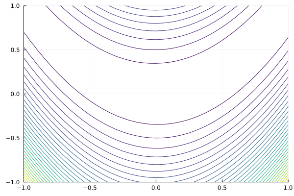
f_r( x, y ) = @. (1.0 - x)^2 + 100.0 * (y - x^2)^2
x_r = -1:0.05:1
y_r = -1:0.05:1
contour( x_r, y_r, f_r.(x_r', y_r ), levels=30, cmap=:viridis, cbar=false )

]add Optim

   Resolving package versions...
   Installed SteadyStateDiffEq ─ v2.0.1
   Installed DiffEqCallbacks ─── v2.37.0
   Installed JumpProcesses ───── v9.14.3
  No Changes to `~/.project/Project.toml`
  No Changes to `~/.project/Manifest.toml`

using Optim

f(x) = (1.0 - x[1])^2 + 100.0 * (x[2] - x[1]^2)^2

f (generic function with 1 method)

x0 = [0.0, 0.0]
res = optimize( f, x0 )

 * Status: success

 * Candidate solution
    Final objective value:     3.525527e-09

 * Found with
    Algorithm:     Nelder-Mead

 * Convergence measures
    √(Σ(yᵢ-ȳ)²)/n ≤ 1.0e-08

 * Work counters
    Seconds run:   0  (vs limit Inf)
    Iterations:    60
    f(x) calls:    117

res.minimizer

2-element Vector{Float64}:
 0.9999634355313174
 0.9999315506115275

res.minimum

3.5255270584829996e-9

?res

search: res red rem Base.rest reset trues read result less keys curves relu repr

res = optimize( f, x0, store_trace = true )

 * Status: success

 * Candidate solution
    Final objective value:     3.525527e-09

 * Found with
    Algorithm:     Nelder-Mead

 * Convergence measures
    √(Σ(yᵢ-ȳ)²)/n ≤ 1.0e-08

 * Work counters
    Seconds run:   0  (vs limit Inf)
    Iterations:    60
    f(x) calls:    117

?res

search: res red rem Base.rest reset trues read result less keys curves relu repr

dump( res.trace )

Array{OptimizationState{Float64, NelderMead{Optim.AffineSimplexer, Optim.AdaptiveParameters}}}((61,))
  1: OptimizationState{Float64, NelderMead{Optim.AffineSimplexer, Optim.AdaptiveParameters}}
    iteration: Int64 0
    value: Float64 0.9506640624999999
    g_norm: Float64 0.045762140642320676
    metadata: Dict{Any, Any}
      slots: Memory{UInt8}
        length: Int64 16
        ptr: Ptr{Nothing} @0x00007f460af06c00
      keys: Memory{Any}
        length: Int64 16
        ptr: Ptr{Nothing} @0x00007f452cd4a8c0
      vals: Memory{Any}
        length: Int64 16
        ptr: Ptr{Nothing} @0x00007f452cd4a960
      ndel: Int64 0
      count: Int64 1
      age: UInt64 0x0000000000000002
      idxfloor: Int64 1
      maxprobe: Int64 0
  2: OptimizationState{Float64, NelderMead{Optim.AffineSimplexer, Optim.AdaptiveParameters}}
    iteration: Int64 1
    value: Float64 0.9506640624999999
    g_norm: Float64 0.020230964744062774
    metadata: Dict{Any, Any}
      slots: Memory{UInt8}
        length: Int64 16
        ptr: Ptr{Nothing} @0x00007f460af06c30
      keys: Memory{Any}
        length: Int64 16
        ptr: Ptr{Nothing} @0x00007f452cd4aa00
      vals: Memory{Any}
        length: Int64 16
        ptr: Ptr{Nothing} @0x00007f452cd4aaa0
      ndel: Int64 0
      count: Int64 1
      age: UInt64 0x0000000000000002
      idxfloor: Int64 1
      maxprobe: Int64 0
  3: OptimizationState{Float64, NelderMead{Optim.AffineSimplexer, Optim.AdaptiveParameters}}
    iteration: Int64 2
    value: Float64 0.9506640624999999
    g_norm: Float64 0.02172171649726186
    metadata: Dict{Any, Any}
      slots: Memory{UInt8}
        length: Int64 16
        ptr: Ptr{Nothing} @0x00007f460af06c60
      keys: Memory{Any}
        length: Int64 16
        ptr: Ptr{Nothing} @0x00007f452cd4ab40
      vals: Memory{Any}
        length: Int64 16
        ptr: Ptr{Nothing} @0x00007f452cd4abe0
      ndel: Int64 0
      count: Int64 1
      age: UInt64 0x0000000000000002
      idxfloor: Int64 1
      maxprobe: Int64 0
  4: OptimizationState{Float64, NelderMead{Optim.AffineSimplexer, Optim.AdaptiveParameters}}
    iteration: Int64 3
    value: Float64 0.9262175083160399
    g_norm: Float64 0.05243757256789791
    metadata: Dict{Any, Any}
      slots: Memory{UInt8}
        length: Int64 16
        ptr: Ptr{Nothing} @0x00007f460af06c90
      keys: Memory{Any}
        length: Int64 16
        ptr: Ptr{Nothing} @0x00007f452cd4ac80
      vals: Memory{Any}
        length: Int64 16
        ptr: Ptr{Nothing} @0x00007f452cd4ad20
      ndel: Int64 0
      count: Int64 1
      age: UInt64 0x0000000000000002
      idxfloor: Int64 1
      maxprobe: Int64 0
  5: OptimizationState{Float64, NelderMead{Optim.AffineSimplexer, Optim.AdaptiveParameters}}
    iteration: Int64 4
    value: Float64 0.8292372137308122
    g_norm: Float64 0.04259748894134015
    metadata: Dict{Any, Any}
      slots: Memory{UInt8}
        length: Int64 16
        ptr: Ptr{Nothing} @0x00007f460af06cc0
      keys: Memory{Any}
        length: Int64 16
        ptr: Ptr{Nothing} @0x00007f452cd4af00
      vals: Memory{Any}
        length: Int64 16
        ptr: Ptr{Nothing} @0x00007f452cd4afa0
      ndel: Int64 0
      count: Int64 1
      age: UInt64 0x0000000000000002
      idxfloor: Int64 1
      maxprobe: Int64 0
  ...
  57: OptimizationState{Float64, NelderMead{Optim.AffineSimplexer, Optim.AdaptiveParameters}}
    iteration: Int64 56
    value: Float64 2.272706709692903e-7
    g_norm: Float64 1.3072092902410254e-7
    metadata: Dict{Any, Any}
      slots: Memory{UInt8}
        length: Int64 16
        ptr: Ptr{Nothing} @0x00007f460af07860
      keys: Memory{Any}
        length: Int64 16
        ptr: Ptr{Nothing} @0x00007f452cd37c20
      vals: Memory{Any}
        length: Int64 16
        ptr: Ptr{Nothing} @0x00007f452cd37e00
      ndel: Int64 0
      count: Int64 1
      age: UInt64 0x0000000000000002
      idxfloor: Int64 1
      maxprobe: Int64 0
  58: OptimizationState{Float64, NelderMead{Optim.AffineSimplexer, Optim.AdaptiveParameters}}
    iteration: Int64 57
    value: Float64 2.120248852111823e-7
    g_norm: Float64 7.108935543504647e-8
    metadata: Dict{Any, Any}
      slots: Memory{UInt8}
        length: Int64 16
        ptr: Ptr{Nothing} @0x00007f460af07890
      keys: Memory{Any}
        length: Int64 16
        ptr: Ptr{Nothing} @0x00007f452cd37ea0
      vals: Memory{Any}
        length: Int64 16
        ptr: Ptr{Nothing} @0x00007f452cd14020
      ndel: Int64 0
      count: Int64 1
      age: UInt64 0x0000000000000002
      idxfloor: Int64 1
      maxprobe: Int64 0
  59: OptimizationState{Float64, NelderMead{Optim.AffineSimplexer, Optim.AdaptiveParameters}}
    iteration: Int64 58
    value: Float64 6.942358374981032e-8
    g_norm: Float64 8.182068301719422e-8
    metadata: Dict{Any, Any}
      slots: Memory{UInt8}
        length: Int64 16
        ptr: Ptr{Nothing} @0x00007f460af078c0
      keys: Memory{Any}
        length: Int64 16
        ptr: Ptr{Nothing} @0x00007f452cd140c0
      vals: Memory{Any}
        length: Int64 16
        ptr: Ptr{Nothing} @0x00007f452cd14160
      ndel: Int64 0
      count: Int64 1
      age: UInt64 0x0000000000000002
      idxfloor: Int64 1
      maxprobe: Int64 0
  60: OptimizationState{Float64, NelderMead{Optim.AffineSimplexer, Optim.AdaptiveParameters}}
    iteration: Int64 59
    value: Float64 1.876333755675703e-8
    g_norm: Float64 2.129209818884303e-8
    metadata: Dict{Any, Any}
      slots: Memory{UInt8}
        length: Int64 16
        ptr: Ptr{Nothing} @0x00007f460af078f0
      keys: Memory{Any}
        length: Int64 16
        ptr: Ptr{Nothing} @0x00007f452cd14200
      vals: Memory{Any}
        length: Int64 16
        ptr: Ptr{Nothing} @0x00007f452cd142a0
      ndel: Int64 0
      count: Int64 1
      age: UInt64 0x0000000000000002
      idxfloor: Int64 1
      maxprobe: Int64 0
  61: OptimizationState{Float64, NelderMead{Optim.AffineSimplexer, Optim.AdaptiveParameters}}
    iteration: Int64 60
    value: Float64 1.876333755675703e-8
    g_norm: Float64 9.270313880771697e-9
    metadata: Dict{Any, Any}
      slots: Memory{UInt8}
        length: Int64 16
        ptr: Ptr{Nothing} @0x00007f460af07920
      keys: Memory{Any}
        length: Int64 16
        ptr: Ptr{Nothing} @0x00007f452cd14340
      vals: Memory{Any}
        length: Int64 16
        ptr: Ptr{Nothing} @0x00007f452cd143e0
      ndel: Int64 0
      count: Int64 1
      age: UInt64 0x0000000000000002
      idxfloor: Int64 1
      maxprobe: Int64 0

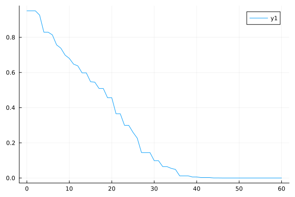
ite = getfield.( res.trace, :iteration )
val = getfield.( res.trace, :value )
plot( ite, val )

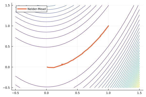
res = optimize( f, x0, store_trace = true, extended_trace=true )

 * Status: success

 * Candidate solution
    Final objective value:     3.525527e-09

 * Found with
    Algorithm:     Nelder-Mead

 * Convergence measures
    √(Σ(yᵢ-ȳ)²)/n ≤ 1.0e-08

 * Work counters
    Seconds run:   0  (vs limit Inf)
    Iterations:    60
    f(x) calls:    117

xs = first.( Optim.centroid_trace(res) );
ys = last.( Optim.centroid_trace(res) );

f_r( x, y ) = @. (1.0 - x)^2 + 100.0 * (y - x^2)^2
x_r = -0.5:0.05:1.5
y_r = -0.5:0.05:1.5
contour( x_r, y_r, f_r.(x_r', y_r ), levels=30, cmap=:viridis, cbar=false )
plot!( xs, ys, lw=4, label="Nelder-Mead" )

x0 = [0.0, 0.0]
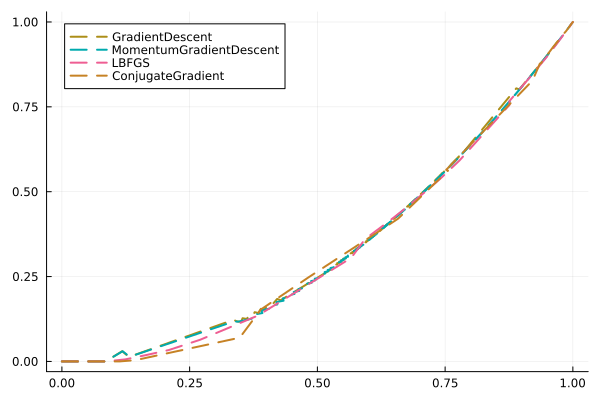
res1 = optimize(f, x0, GradientDescent(), Optim.Options(store_trace=true, extended_trace=true) );
res2 = optimize(f, x0, MomentumGradientDescent(), Optim.Options(store_trace=true, extended_trace=true) );
res3 = optimize(f, x0, LBFGS(), Optim.Options(store_trace=true, extended_trace=true) );
res4 = optimize(f, x0, ConjugateGradient(), Optim.Options(store_trace=true, extended_trace=true) );

plot( first.( Optim.x_trace(res1) ), last.( Optim.x_trace(res1) ), lw=2, ls=:dash, c=5, label="GradientDescent" )
plot!( first.( Optim.x_trace(res2) ), last.( Optim.x_trace(res2) ), lw=2, ls=:dash, c=6, label="MomentumGradientDescent" )
plot!( first.( Optim.x_trace(res3) ), last.( Optim.x_trace(res3) ), lw=2, ls=:dash, c=7, label="LBFGS" )
plot!( first.( Optim.x_trace(res4) ), last.( Optim.x_trace(res4) ), lw=2, ls=:dash, c=8, label="ConjugateGradient" )

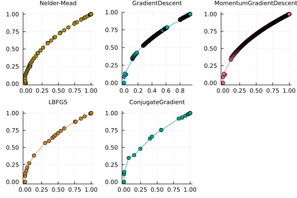
plot(
    plot( last.( Optim.centroid_trace(res) ), first.( Optim.centroid_trace(res) ), c=5, title="Nelder-Mead", markershape=:circle ),
    plot( last.( Optim.x_trace(res1) ), first.( Optim.x_trace(res1) ), c=6, title="GradientDescent", markershape=:circle ),
    plot( last.( Optim.x_trace(res2) ), first.( Optim.x_trace(res2) ), c=7, title="MomentumGradientDescent", markershape=:circle ),
    plot( last.( Optim.x_trace(res3) ), first.( Optim.x_trace(res3) ), c=8, title="LBFGS", markershape=:circle ),
    plot( last.( Optim.x_trace(res4) ), first.( Optim.x_trace(res4) ), c=9, title="ConjugateGradient", markershape=:circle ),
    leg=false, titlefont=font(8)
)

Создаем полиномы

]add Polynomials

using Polynomials

]add CSV

using CSV, DataFrames
data_df = CSV.read("Filip.csv", header=true, delim=' ', ignorerepeated=true, DataFrame );
coeffs_df = CSV.read("Filip_coeffs.csv", header=true, delim=' ', ignorerepeated=true, DataFrame );

extrema(data_df.x)

(-8.781464495, -3.13200249)

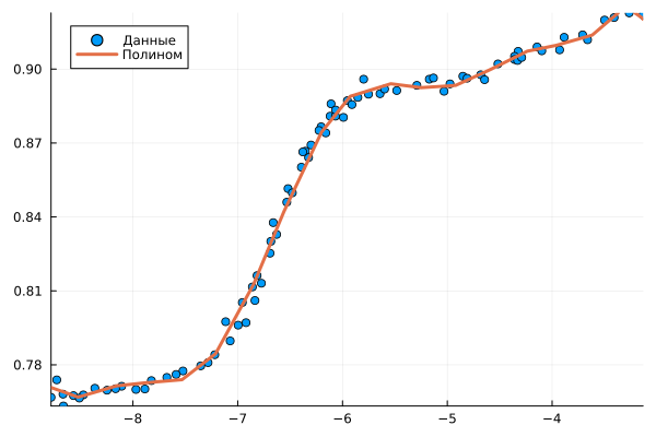
scatter( data_df.x, data_df.y, label="Данные" )
plot!( Polynomial(coeffs_df.Estimate), lw=3, label="Полином" )
plot!( xlimits=extrema(data_df.x), ylimits=extrema(data_df.y) )

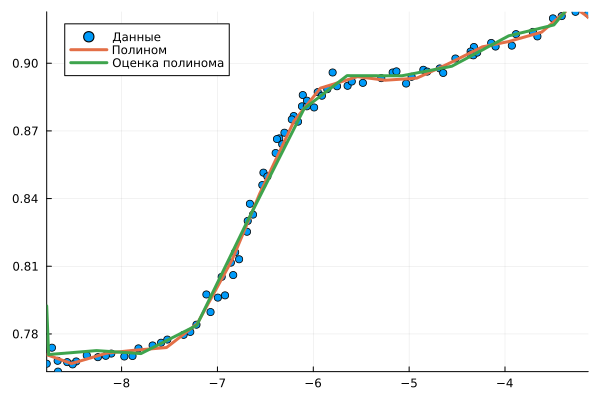
p = Polynomials.fit( data_df.x, data_df.y, 10 )

plot!( p, lw=3, label="Оценка полинома" )
plot!( xlimits=extrema(data_df.x), ylimits=extrema(data_df.y) )

]add GLM

using GLM
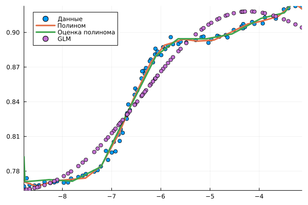
p_lm = lm( @formula( y ~ sin(x) + x^2), data_df )

StatsModels.TableRegressionModel{LinearModel{GLM.LmResp{Vector{Float64}}, GLM.DensePredChol{Float64, LinearAlgebra.CholeskyPivoted{Float64, Matrix{Float64}, Vector{Int64}}}}, Matrix{Float64}}

y ~ 1 + :(sin(x)) + :(x ^ 2)

Coefficients:
────────────────────────────────────────────────────────────────────────────────
                  Coef.   Std. Error       t  Pr(>|t|)    Lower 95%    Upper 95%
────────────────────────────────────────────────────────────────────────────────
(Intercept)   0.922318   0.00653498   141.14    <1e-95   0.90931      0.935325
sin(x)        0.0318398  0.00429341     7.42    <1e-09   0.023294     0.0403857
x ^ 2        -0.0018094  0.000159772  -11.32    <1e-17  -0.00212741  -0.00149138
────────────────────────────────────────────────────────────────────────────────

scatter!( data_df.x, GLM.predict( p_lm, data_df ), lw=3, label="GLM" )
plot!( xlimits=extrema(data_df.x), ylimits=extrema(data_df.y))

Обучим нейросеть

]add Flux

using Flux

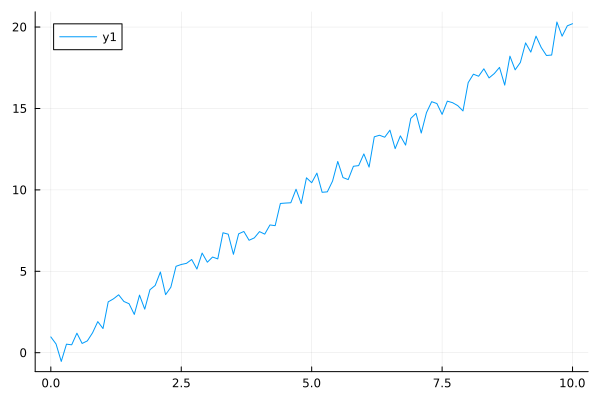
Xs = Float32.( 0:0.1:10 )
Ys = Float32.( 2Xs .+ 2(rand(length(Xs)).-0.5) )
plot( Xs, Ys )

model = Dense( 1 => 1 )

Dense(1 => 1)       # 2 parameters

loss(x,y) = Flux.mse(model(x), y)

loss (generic function with 1 method)

opt = Flux.Adam(0.1)

Flux.Optimise.Adam(0.1, (0.9, 0.999), 1.0e-8, IdDict{Any, Any}())

data = [(Xs', Ys')]

1-element Vector{Tuple{LinearAlgebra.Adjoint{Float32, Vector{Float32}}, LinearAlgebra.Adjoint{Float32, Vector{Float32}}}}:
 ([0.0 0.1 … 9.9 10.0], [0.9708044 0.5367785 … 20.076197 20.20464])

model( [1] )

1-element Vector{Float32}:
 -1.4566025

for i in 1:1000
    Flux.train!( loss, Flux.params(model), data, opt )
end

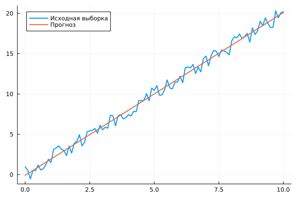
X_прогноз = [ [x] for x in Xs ]
Y_прогноз = model.( X_прогноз )

plot( Xs, Ys, label="Исходная выборка", legend=:topleft, lw=2 )
plot!( Xs, vec(hcat(Y_прогноз...)), label="Прогноз", lw=2 )

model.weight

1×1 Matrix{Float32}:
 -1.3400369

model.bias

1-element Vector{Float32}:
 0.0

using Symbolics
@variables x1
model( [x1] )

Многослойная нейросеть

model = Chain(  Dense(1=>4, relu), Dense(4=>2, sigmoid), Dense(2=>1) )

Chain(
  Dense(1 => 4, relu),                  # 8 parameters
  Dense(4 => 2, σ),                     # 10 parameters
  Dense(2 => 1),                        # 3 parameters
)                   # Total: 6 arrays, 21 parameters, 396 bytes.

@variables x1
model( [x1] )

#]add ChainPlots

#using ChainPlots

#gr()
#plot( model )

Классификатор

model = Dense( 1=>2 )

Dense(1 => 2)       # 4 parameters

loss(x,y) = Flux.crossentropy( model(x), y )

loss (generic function with 1 method)

?Flux.crossentropy

Вычисления на GPU

using CUDA

# CUDA.set_runtime_version!(v"12.2")

@time CUDA.rand( 10000,10000 ).^2;

@time CUDA.rand( 10000,10000 ).^2;

@time rand( 10000,10000 ).^2;

@time rand( 10000,10000 ).^2;

CUDA.functional()

Задачи для изучения синтаксиса

Найти минимум функции f(x) = (x - 3)^2 + 5 с помощью градиентного спуска.

using Optim
f(x) = (x[1] - 3)^2 + 5  # x передается как массив, даже если он из одного элемента
result = optimize(f, [0.0]) # Начинаем поиск с x = 0
println("Минимум найден в x = ", result.minimizer[1], " значение f = ", result.minimum)

Обучить однонейронную сеть (линейную регрессию) предсказывать y = 2x + 1.

using Flux, Statistics
# 1. Создаем данные: y = 2x + 1 + небольшой шум
x = rand(100) * 10
y = 2 .* x .+ 1 .+ randn(100)

# 2. Создаем модель: один полносвязный слой без активации (линейная регрессия)
model = Dense(1 => 1)

# 3. Функция потерь
loss(x, y) = Flux.mse(model(x), y)

# 4. Данные и оптимизатор
data = [(x[i],y[i]) for i in 1:100]
opt = Descent(0.01) # Gradient descent with learning rate 0.01

# 5. Цикл обучения
for epoch in 1:100
    Flux.train!(loss, Flux.params(model), data, opt)
end

# Смотрим, чему равны оценки веса и смещени
println("Веса: ", model.weight)
println("Смещение: ", model.bias)
# Должны быть близки к 2 и 1

День 4 Летней школы Julia

Поиск минимума

Создаем полиномы

Обучим нейросеть

Многослойная нейросеть

Классификатор

Вычисления на GPU

Задачи для изучения синтаксиса

Тип

Краткое описание

Связанные материалы

Теги

Категории

Языки

Форматы

Уровень

Статус

Опубликовано

Обновлено

Источник